Kirchhoff’s Laws
You will apply Kirchhoff’s current law at a node and Kirchhoff’s voltage law around a loop. These laws let you write equations for a circuit that cannot be reduced by inspection.
Used in college or university: Nodal analysis, mesh analysis, electronics, power systems, and control hardware. [1, Ch. 9]
Where you see it: In a car wiring harness, current splits between lights and control modules. In a robot, it splits between the controller, sensors, and motors.
The bottom rail is normally the 0 V or ground reference, and higher-voltage nodes are drawn above it. On a vertical battery symbol, the long line is positive. Keep that polarity consistent with every current arrow and voltage sign when writing Kirchhoff equations.
Class materials
- Teaching slides
- Assignment: From Two Loops to a Matrix
- Printable two-loop-to-matrix guide
- Make a copy of the current student problem set
- TEJ Electronics Quick Reference
- Make a copy of the General Schematic and GUESS handout
- Grob Chapter 9: Kirchhoff’s Laws
- Grob Problems Manual for Chapter 9 practice
- ElectroBOOM101-008: Lumped Model, Kirchhoff Circuit Laws
- Teacher answers: restricted
Watch ElectroBOOM101-008 together as the unit capstone rather than restarting the completed assignment. While watching, record one statement about the lumped-circuit model, one KCL statement, and one KVL statement. The teacher will then use the completed Question 4 equations to introduce standard form, the matrix equation \(A\mathbf{x}=\mathbf{b}\), numpy.linalg.solve, negative-current interpretation, and residual verification. Predict each result before the live code runs. Monday is for explanation, prediction, and questions; the independent lab is Tuesday.
Tuesday: derive two loops, build the matrix, and solve two ways
Open the complete student assignment and submission instructions, use the printable two-loop guide, and download Notebook 3A. Use the completed Question 4 circuit and its released answer. This is not another KCL/KVL worksheet. It teaches the missing bridge from loop traversal to standard form and a matrix.
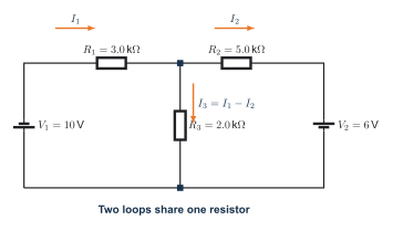
- Define \(I_1\), \(I_2\), and the shared current \(I_3=I_1-I_2\).
- Walk around Loop 1 and explain every KVL sign before rearranging Equation 1.
- Walk around Loop 2 and explain why the shared-resistor sign changes before rearranging Equation 2.
- State the variable order and units, build \(A\) and \(\mathbf{b}\), and read both matrix rows back as equations.
- Solve numerically with
numpy.linalg.solveand report the residual vector. - Solve symbolically with
sympy.solve, preserve the exact fractions, and calculate \(I_3\). - Compare the original, released, numerical, and symbolic results, then complete the reflection.
Tuesday submission: one completed .ipynb file containing both full loop derivations, the matrix, NumPy results and residuals, SymPy exact results, the comparison table, and the assigned reflection. No physical lab or new circuit topology is required while the regular teacher is absent.
Do not compress the debugging ladder into Tuesday. Notebook 3 later uses a keyword error, a non-square numpy.linalg.solve input, and a silent factor-of-1000 unit bug. The parameter sweep is also later. Tomorrow is only the two-loop derivation, matrix, numerical solution, symbolic solution, and verification.
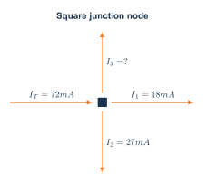
Kirchhoff’s current law
\[ \sum I_{\mathrm{in}} = \sum I_{\mathrm{out}} \tag{1}\]
A negative answer means the real current is opposite the arrow you selected.
Kirchhoff’s voltage law
\[ \sum_{k=1}^{n}\Delta V_k = 0 \tag{2}\]
Choose one loop direction and keep the signs consistent. A source rise is positive; a resistor drop in the current direction is negative.
Workflow
- Mark the essential nodes and independent loops.
- Choose and label unknown current directions.
- Write current-law and voltage-law equations.
- Replace resistor voltage with \(V=IR\).
- Solve without rounding, then check every original node and loop equation.
- Build the same network in Tinkercad and compare the simulated values.
Worked solutions
Kirchhoff’s voltage law requires the source rise to equal the voltage drops:
\[ V_3=12.0\,\mathrm{V}-2.4\,\mathrm{V}-4.1\,\mathrm{V}=5.5\,\mathrm{V}. \tag{3}\]
Check: \(12.0-2.4-4.1-5.5=0.0\,\mathrm{V}\).
The two loop equations are
\[ 5I_1-2I_2=10 \tag{4}\]
\[ -2I_1+7I_2=6. \tag{5}\]
Solving them gives \(I_1=2.645161\ldots\,\mathrm{mA}\) and \(I_2=1.612903\ldots\,\mathrm{mA}\).
The shared-branch current is
Final answers: \(I_1=2.65\,\mathrm{mA}\), \(I_2=1.61\,\mathrm{mA}\), and \(I_3=1.03\,\mathrm{mA}\).
Practical pathway: test the node and loops
Core learning: derive the node and loop equations by hand before using a simulator or solver. Follow Define Variables → Write Equations → Standard Form or Matrix → Solve → Verify.
Guided practice: if Tinkercad can represent the same sources and passive components faithfully, build the two-loop network with the Tinkercad tutorial. Otherwise, use the teacher-approved physical circuit or simulator and identify the substitution. Measure the currents needed for one KCL check and voltages needed for one KVL check.
| Check | Predicted total | Simulated or measured total | Residual |
|---|---|---|---|
| Current entering minus leaving (mA) | 0 | ||
| Left-loop voltage sum (V) | 0 | ||
| Right-loop voltage sum (V) | 0 |
Independent challenge: deliberately reverse one current arrow without changing the circuit. Rewrite the affected signs, solve again, and explain why a negative result is meaningful rather than automatically wrong.
- Keep one chosen loop direction from start to finish.
- Compare every matrix row with its original KCL or KVL equation.
- A residual near zero checks the entered equations; compare signs and units with the schematic to check the model.
Use Notebook 3 only after deriving the equations. Record the coefficient order and verify by substitution.
Reflection: What did the residual establish, and what mistake could still produce a near-zero residual?