Parallel Circuits
You will identify parallel branches and calculate equivalent resistance, source current, branch current, and power. This explains how several loads can operate independently from one source.
Used in college or university: Circuit analysis, electrical distribution, instrumentation, and electronics.
Where you see it: A car connects lights and control modules in parallel so each receives battery voltage. A robot does the same when several sensors share one supply.
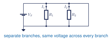
Higher voltage is at the top and the 0 V or ground return is at the bottom. The battery’s long line is the positive terminal. Conventional current leaves the positive rail, divides between the branches, and returns to ground.
Class materials
Package 1: Basic Electricity to Computer Loads
- Teaching slides
- Make a copy of the parallel-circuit calculations handout
- Make a copy of the circuit-calculations photo submission
- Student models for Questions 1 and 2
Package 2: Parallel Review and Series Circuits
- Teaching slides
- Make a copy of the six-question student problem set
- Student worked models for Questions 2 and 4
- Series-circuit notes
- Sigma notation LaTeX source
Core references
- TEJ Electronics Quick Reference
- Standard 5% resistor values, page 2
- Make a copy of the General Schematic and GUESS handout
- Teacher answers: restricted
Textbook and laboratory support
- Grob Chapter 5: Parallel Circuits - the main reference for branch voltage, current, resistance, and power.
- Grob Problems Manual - solved examples and additional Chapter 5 practice.
- Experiment 5-1: Parallel Circuits - build and verify the common-voltage rule.
- Experiment 5-2: Parallel Circuits - Resistance Branches - optional resistance extension.
- Experiment 5-3: Parallel Circuits - Analysis - optional complete-analysis extension.
Common voltage
Components are in parallel when both ends connect to the same two nodes. Every branch has the same voltage:
\[ V_k = V_T \tag{1}\]
General parallel rules
The source current is the sum of the branch currents:
\[ I_T = \sum_{k=1}^{n} I_k \tag{2}\]
The equivalent resistance is
\[ \frac{1}{R_T} = \sum_{k=1}^{n}\frac{1}{R_k} \tag{3}\]
For exactly two parallel resistors, the product-over-sum shortcut is
\[ R_T = \frac{R_aR_b}{R_a+R_b} \tag{4}\]
Calculate any branch current with Ohm’s law:
\[ I_k = \frac{V_T}{R_k} \tag{5}\]
Total power equals the sum of the branch powers:
\[ P_T = \sum_{k=1}^{n}P_k = V_T I_T \tag{6}\]
How sigma notation works
\[ I_T=\sum_{k=1}^{n}I_k=I_1+I_2+\cdots+I_n \tag{7}\]
\[ \frac{1}{R_T}=\sum_{k=1}^{n}\frac{1}{R_k} =\frac{1}{R_1}+\frac{1}{R_2}+\cdots+\frac{1}{R_n} \tag{8}\]
| Symbol | Meaning |
|---|---|
| \(R_T\) or \(R_{eq}\) | total or equivalent resistance |
| \(R_k\) or \(I_k\) | the value at position \(k\) |
| \(k\) | the index variable; it changes through \(1,2,3,\ldots,n\) |
| \(n\) | the fixed last index; the sum stops here |
\(\Sigma\) means add each term while \(k\) runs from \(1\) to \(n\). The final expanded term uses \(n\).
Check the answer
\[ \sum_{k=1}^{n} I_k \overset{?}{=} I_T \tag{9}\]
Equation Equation 9 checks the branch currents. The equivalent resistance from Equation Equation 3 must be smaller than the smallest branch resistance.
Practical pathway: one branch changes
Core learning: complete the existing parallel-circuit questions first. Then follow the Tinkercad build and measurement tutorial to reproduce a two-branch circuit from this lesson.
Guided practice: predict the source current and both branch currents. Simulate the circuit and measure the common branch voltage plus each current. Stop the simulation before changing a resistor.
| Quantity and location | Predicted | Simulated | Difference |
|---|---|---|---|
| Common branch voltage (V) | |||
| Branch 1 current (mA) | |||
| Branch 2 current (mA) | |||
| Source current (mA) |
Independent challenge: increase one branch resistance to another available value. Predict which quantities will change and which will stay constant before restarting. Verify that branch currents add to source current.
- Both branches still connect to the same two nodes.
- Review common voltage and the current-sum check above.
- Recalculate only the changed branch current, then add the branch currents for the new source current.
Optional Python verification: use Notebook 2 when you want to compare several branch values efficiently.
Reflection: What did the unchanged quantity reveal about parallel topology? What wiring or unit error would break your current-sum check?
Question 1 in the review problem set is the parallel review. Teachers can email Andrew for the complete answer key.
These notes follow Grob’s Basic Electronics, Chapter 5. [1, Ch. 5]