Capacitors 3: RC Time Constants and Design
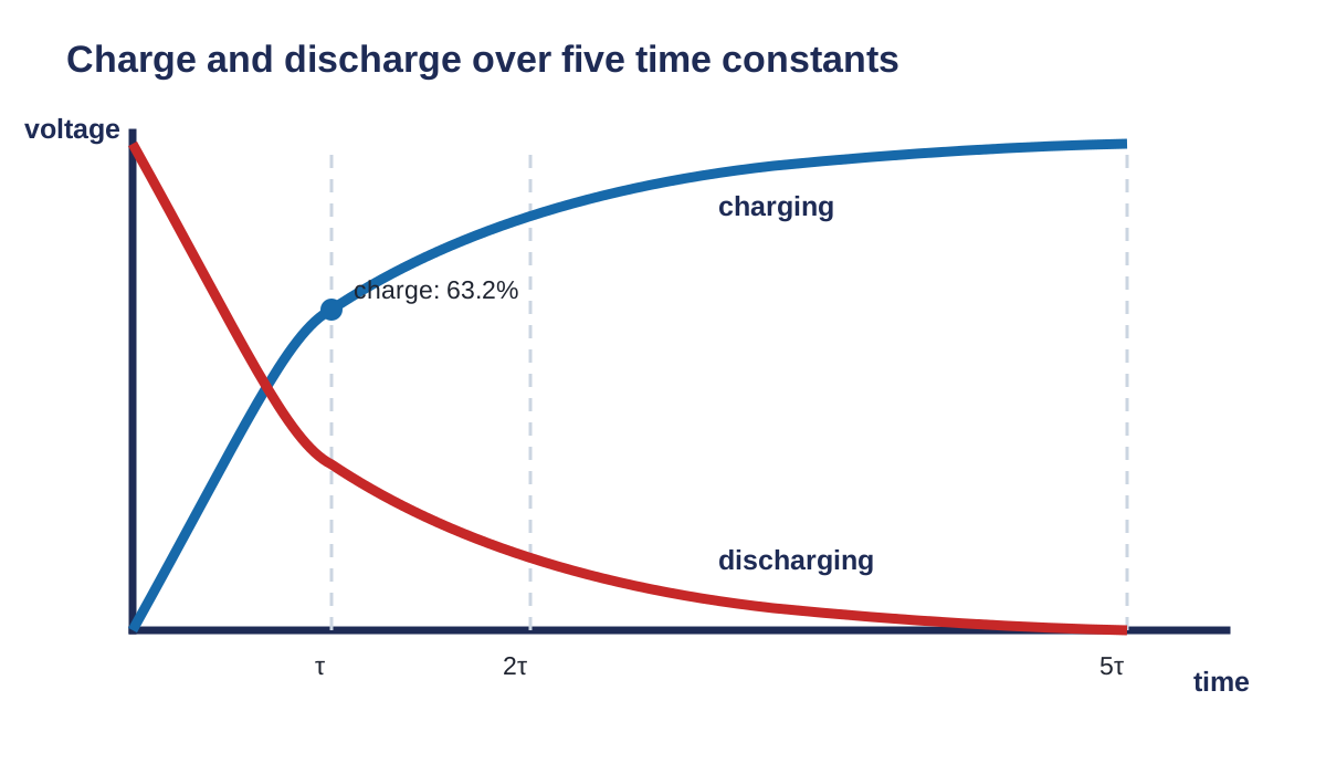
This lesson turns the charging curve into a design tool. Start with a target time, choose \(R\) and \(C\), then check the actual result.
The time constant
For a simple resistor-capacitor circuit:
\[ \tau=RC \]
where:
- \(\tau\) is time in seconds;
- \(R\) is resistance in ohms;
- \(C\) is capacitance in farads.
Useful unit combinations are:
\[ \mathrm{k\Omega}\times\mathrm{\mu F}=\mathrm{ms}, \qquad \mathrm{M\Omega}\times\mathrm{\mu F}=\mathrm{s} \]
Worked example using GUESS
A circuit uses \(R=15\,\mathrm{k\Omega}\) and \(C=47\,\mu\mathrm{F}\). Calculate the time constant and the practical charging time.
Given
\[R=15\,000\,\Omega,\qquad C=47\times10^{-6}\,\mathrm{F}\]
Unknown
\[\tau=?,\qquad 5\tau=?\]
Equation
\[\tau=RC\]
Substitute and solve
\[ \tau=(15\,000\,\Omega)(47\times10^{-6}\,\mathrm{F})=0.705\,\mathrm{s} \]
\[ 5\tau=5(0.705\,\mathrm{s})=3.525\,\mathrm{s} \]
Statement
The time constant is \(0.705\,\mathrm{s}\), and practical charging takes about \(3.53\,\mathrm{s}\).
Use the time scale on the graph
Solve for a part value
If the target time and capacitance are known:
\[ R=\frac{\tau}{C} \]
If the target time and resistance are known:
\[ C=\frac{\tau}{R} \]
The exact answer may not be a standard part value. Choose an available part and recalculate the actual time constant.
Example: a target of \(2.00\,\mathrm{s}\) with \(R=22.0\,\mathrm{k\Omega}\) requires:
\[ C=\frac{2.00\,\mathrm{s}}{22\,000\,\Omega}=90.9\,\mu\mathrm{F} \]
A \(100\,\mu\mathrm{F}\) part gives:
\[ \tau=(22.0\,\mathrm{k\Omega})(100\,\mu\mathrm{F})=2.20\,\mathrm{s} \]
State both the ideal calculated value and the actual value from the selected part.
Optional calculus bridge
You do not need calculus to complete this lesson. The full ideal equations are:
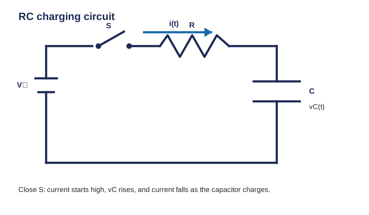
\[ v_C(t)=V_S\left(1-e^{-t/RC}\right) \]
for charging, and:
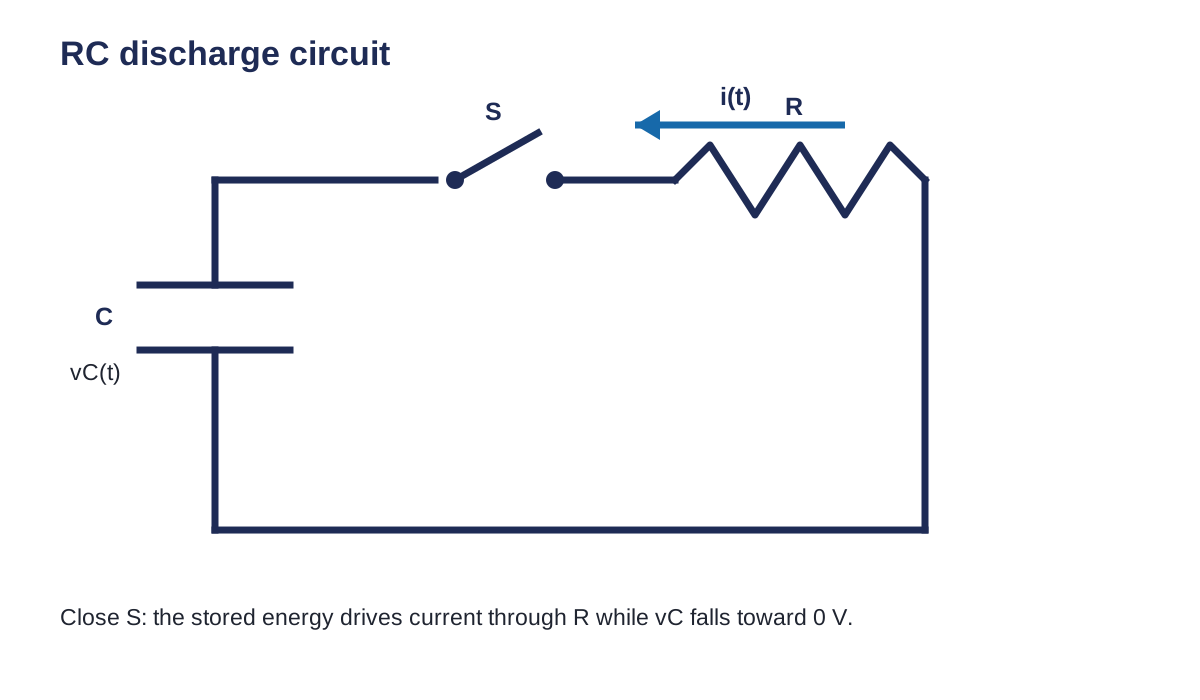
\[ v_C(t)=V_0e^{-t/RC} \]
for discharging.
Differentiation describes how fast voltage changes. Integration connects current over time to stored charge. Later, an op amp can build practical integrators and differentiators.
Jupyter and Tinkercad check
- Calculate \(\tau\) and \(5\tau\) by hand.
- Run the notebook with the same \(R\), \(C\), and source voltage.
- Double \(R\) and predict the change before running the cell.
- Reset \(R\), double \(C\), and compare.
- Build one assigned circuit in Tinkercad.
- Measure \(v_C\) near one time constant and compare it with \(0.632V_S\).
Complete the work
- Complete all five questions using GUESS.
- Show the unit conversions.
- Use the notebook to verify each numerical result.
- Build Question 4 or 5 in Tinkercad.
- Submit the sheet, notebook, and Tinkercad link.
Textbook support: Grob, Chapter 22, pp. 668-691. Practice support: Problems Manual, Chapter 22, pp. 309-316. Optional teacher-approved lab: Experiment 22-1. [1, Ch. 22]
Equation and diagram source files
Where this leads
Continue to Diodes and LEDs, then Transistors, and then Operational Amplifiers and the XL741. Capacitors and resistors also lead to filters, integrators, differentiators, and calculus.
Help improve this lesson
If a direction, calculation, simulation step, or code cell is unclear, identify the exact step. Explain what you tried and what happened.