Results from Modeling a Thermister
In the last blog post, I described a long winded approach about how I built a model for a thermister to relate the voltage measured from a BeagleBoneBlack (BBB) microcontroller to the temperature. This post will summarize the results from the model, and explain how to connect up the system.
Thermal Sensor Data
The thermal sensor used is a 100k thermistor Part No. HT100K3950-1 invidually connected to a 1m cable:
Hotend Thermistor
100K Glass-sealed Thermistor
3950 1% thermistor 1.8mm glass head
1M long cables 2 wires
PTFE Tube 0.6*1mm to protect from the thermistor
Shrink wrap between thermistor and the cables.
The site included a weird word document with a bunch of numbers. I saved the data as a .csv file so I can use the data in python. If you want to follow along, you can you download the document here
I then made a chart which includes the expected resistance and the errors. This chart summarizes the data provided by the manufacturer:
#import necessary libraries:
import pandas as pd
import numpy as np
import pylab as P
import plotly.plotly as py

import math
from scipy.optimize import curve_fit
import matplotlib.pyplot as plt
import matplotlib.mlab as mlab
import matplotlib.gridspec as gridspec
#comment below if not using ipython/jupyter notebook
%matplotlib inline

#read csv and label columns
data = pd.read_csv('100k-thermistor.csv')
data.columns = ['temperature', 'r_max', 'r_norm','r_min']

data['lower_error'] = data.r_norm-data.r_min
data['upper_error'] = data.r_max-data.r_norm

asymmetric_error = [data.lower_error, data.upper_error]

fig1 = plt.figure(1)
plt.plot(data.temperature, data.r_norm,color='k', label='expected resistance')
plt.title('Expected Resistance vs Temperature')
plt.xlabel("Temperature (degrees C)")
plt.ylabel("Resistance (kohm)")
#plt.show()
#py.iplot_mpl(fig1)
fig2 = plt.figure(2)
plt.plot(data.temperature,data.r_min-data.r_norm, label='lower error')
plt.plot(data.temperature,data.r_max-data.r_norm, label='upper error')
plt.title("Upper and Lower Error vs Temperature")
plt.xlabel("Temperature (Celcius)")
plt.ylabel("Resistance (kohm)")
#py.iplot_mpl(fig2)We than then limit the data to operating temperature range which I care about:
#set the desired upper and lower temperature
lower_temp_range = 19
upper_temp_range = 81

#starting_temp sets the index adjustement for array
starting_temp = data.temperature[0]

selected_temp = data.temperature[lower_temp_range-starting_temp:upper_temp_range-starting_temp]
selected_r_norm = data.r_norm[lower_temp_range-starting_temp:upper_temp_range-starting_temp]

fig1 = plt.figure(1)
plt.plot(selected_temp, selected_r_norm,color='k', label='expected resistance')
plt.title('Expected Resistance vs Temperature')
plt.xlabel("Temperature (degrees C)")
plt.ylabel("Resistance (kohm)")
#plt.show()

#this makes an interative plot using plotly
#py.iplot_mpl(fig1)
selected_r_min = data.r_min[lower_temp_range-starting_temp:upper_temp_range-starting_temp]
selected_r_max = data.r_max[lower_temp_range-starting_temp:upper_temp_range-starting_temp]
fig2 = plt.figure(2)
plt.plot(selected_temp,selected_r_min-selected_r_norm, label='lower error')
plt.plot(selected_temp,selected_r_max-selected_r_norm, label='upper error')
plt.title("Upper and Lower Error vs Temperature")
plt.xlabel("Temperature (Celcius)")
plt.ylabel("Resistance (kohm)")
#comment if not using plotly
#py.iplot_mpl(fig2)Based on the Resistance vs Temperature Chart, we can make an assumption that the distribution follows the relationship followed by this fitness function:
\(resistance = a e^{-b \times temperature} + c\) where resistance is meaured in \(k\Omega\), temperature measued in degrees celcius, and the constants a, b, and c can be found (through curve fitting).
Lets define the fitness function and find the constants a, b, and c.
def fitness_function(temperature, a, b, c):
    return a*np.exp(-b*temperature) + c # kohm

selected_temp_fit_parms, selected_temp_fit_covariances = curve_fit(fitness_function,
                                                    selected_temp, selected_r_norm)
print ' fit coefficients:\n', selected_temp_fit_parms, '\n'
print 'a=',selected_temp_fit_parms[0],'\n'
print 'b=',selected_temp_fit_parms[1],'\n'
print 'c=',selected_temp_fit_parms[2],'\n'

print ' Covariance matrix:\n', selected_temp_fit_covariances

selected_temp_fit = fitness_function(selected_temp,
                                 selected_temp_fit_parms[0],
                                 selected_temp_fit_parms[1],
                                 selected_temp_fit_parms[2])
residual_error_selected = selected_temp_fit-selected_r_norm

fig3 = plt.figure(1)
plt.plot(selected_temp, selected_temp_fit,label='curve fit', color='k')
plt.xlabel("Temperature (Celcius)")
plt.ylabel("Resistance (kohm)")
plt.title("Curve Fit Resitance vs Temperature")

#py.iplot_mpl(fig3)
fit coefficients:
[ 2.95517151e+02 4.52495454e-02 5.12190680e+00]
a= 295.517150959
b= 0.0452495454444
c= 5.12190680215
Covariance matrix:
[[ 6.94401115e-01 1.20117237e-04 8.77447476e-02]
[ 1.20117237e-04 2.41377772e-08 2.04485474e-05]
[ 8.77447476e-02 2.04485474e-05 2.05394937e-02]]
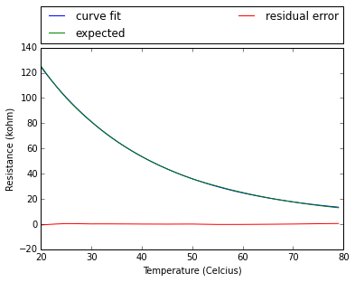
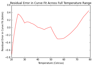
Now lets plot the expected resistance, curve fit resistance and residuals to understand the error in the curve fit:
plt.figure(2)
plt.plot(selected_temp, selected_temp_fit,label='curve fit')
plt.plot(selected_temp, selected_r_norm, label='expected')
plt.plot(selected_temp,residual_error_selected, 'r' , label='residual error')
plt.legend(bbox_to_anchor=(0., 1.02, 1., .102), loc=3,
           ncol=2, mode="expand", borderaxespad=0.)
plt.xlabel("Temperature (Celcius)")
plt.ylabel("Resistance (kohm)")

plt.figure(3)
plt.plot(selected_temp,residual_error_selected, 'r' , label='residual error')
plt.xlabel("Temperature (Celcius)")
plt.ylabel("Residual Error in Curve Fit (kohm)")
plt.title("Residual Error in Curve Fit Across Full Temperature Range")

plt.figure(4)
# convert numpy series to array
residual_error_list  = residual_error_selected.tolist()
residual_error_array = np.asarray(residual_error_list)

error_mean = np.mean(residual_error_array)
error_sigma = np.std(residual_error_array)
print "Residual mean (Kohm):"
print error_mean
print "Residual std dev (Kohm):"
print error_sigma


n, bins, patches = plt.hist(residual_error_array, 50, normed=1, facecolor='red', alpha=0.75)
plt.xlabel("Error in Curve fit (kohm)")
plt.title("Residual Distribution")
y = P.normpdf( bins, error_mean, error_sigma)
l = P.plot(bins, y, 'k--', linewidth=1.5)
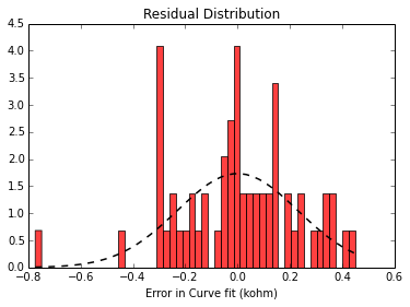
Residual mean (Kohm):
-8.15077359012e-09
Residual std dev (Kohm):
0.264370345418


As we can see, the residual error is very small compared to the range of resistance, and follows a (some what) normal distribution. That we have a model of resistance vs temperature, lets set up our microcontroller (BBB) to measure temperature. Since our sensor is a variable resistor, we can take an analog mesaurement by passing a current though the thermister and measuring the voltage accross it. Since we need to limit our input voltage to 1.8 V (according to the BBB spec, we can use a voltage divider to limit the maximum voltage accross the thermistor (as shown below)
In our case, we need to calculate the correct R1 to ensure the voltage accross the thermistor (which is read through the analog input pin of the BBB) does not exceed 1.8V based on the maximum operating range of temperature. For us this is between 0C and 100 C. Based on the plot of the resistance vs temperature for the thermistor, we know that at 0C, the resistance of the thermistor is a maximum of 327.240 Kohm. We can then use this value as R2 in a generic voltage divider, to calculate for R1.
\[R_1 = R_2 \frac{V_{in}}{V_o} - R_2\]v_in = 3.3 #V
v_out = 1.8 #V
r_2_max = 327260 #ohm
r_1 = r_2_max * v_in / v_out - r_2_max #ohm
print "Minimum value for R1 in kohms"
print r_1 /1000 #kohmMinimum value for R1 in kohms
272.716666667
Looking at the standard 1% resistor chart or calculator we now know we should use 274k ohm resistor for R1.
Now that we have R1 and Vin set as constants and we can measure Vo from the BBB’s analog input pin, we can now write a rearrange the voltage divider equation and fitness function to relate Vo to temperature. The previous blog post goes over this, but the resulting function is here:
def voltage_to_temperature(voltage_reading):
    #calculated to limit input voltage 1.8V max
    v_in = 3.3 #Volts

    r_1 = 274 #kohm

    #taken by curve fitting
    a = 2.94311453*pow(10,2)
    b = 4.51009053*pow(10,-2)
    c = 5.054388390

    #taken from voltage divider equation
    r_2 = r_1 * voltage_reading / (v_in - voltage_reading) # kohm

    #taken from rearraging fitness function
    #solve r_2 = a*np.exp(-b*temperature) + c) for t
    t = -1 * (np.log((r_2-c)/a))/b #degrees C
    return t
We can now use this function and plot for the full range of input voltages:
v_measured_min = 0 #V
v_measured_max = 1.8 #V
v_sweep = np.linspace(v_measured_min, v_measured_max, num=1000)
temperature_profile = voltage_to_temperature(v_sweep)

fig = plt.figure(1)
plt.plot(v_sweep, temperature_profile)
plt.ylabel("Temperature (Celcius)")
plt.xlabel("Measured Voltage (V)")
plt.title("Temperature vs Measured Voltage")

#py.iplot_mpl(fig)