In the last blog post, I talked about voltage dividers and how they can be used to limit voltage to eventually connect to an ADC to measure voltage on a BeagleBone. Today I am going to build on the voltage divider and pair hardware engineering with data science. The next couple of posts will be pieces of battery testing rig, and then I will put it all togeather to explain how the full system works. First things first, what temperature sensor should we use?

Selecting a Thermal Sensor

Half due to avaliability, and the other half due to shear laziness (of not wanting to buy sensors), I decided we are going to use thermisters as our temperature sensor of choice. A friend hand a bunch so why use them?

Specifically, he gave me a bunch of 100k thermistors Part No. HT100K3950-1 invidually connected to a 1m cable.

What is a thermister?

A thermister can be simply defined as a special type of resistor whose resistance is highly dependent on temperature. Therefore if you are able to measure the resistance on the thermister, you can easily determine the temperature if you know how the thermister behaves. Simple enough right?

If you go to the site which sells them, they give a bit more information:

Hotend Thermistor 100K Glass-sealed Thermistor 3950 1% thermistor 1.8mm glass head
1M long cables 2 wires
PTFE Tube 0.6*1mm to protect from the thermistor
Shrink wrap between thermistor and the cables.

The most important piece of information to get started using the thermister is its behaviour responding to temperature. Luckly for me, my friend sent me the data which was on the site. When you have a table or chart which maps the resistance to temperature, you can simply measure the resistance with a multimemter and look up the temperature on the chart, or you can again use a voltage divider and connect it to an ADC (more on that later).

Mapping Resistance to Temperature using Curve Fitting

The site included a weird word document with a bunch of numbers. It really confuses me why one would have tabular data in a word document, a spreadsheet serves that purpose. Anyways, the information was easily extractable and I was able to put it into an spreadsheet and save as a .CSV file. If you want to follow along, you can you download the document here

Once you own the file in a speadsheet program or in your text editor of choice, you can see there are four columns: temperature in Celcius, maximum resistance in $k\Omega$, normal (average)resistance in $k\Omega$ and minimum resistance in $k\Omega$ . If we were measuring the resistance by hand, we could simply just look up (and eyeball) the closest resistance value and read of the temperature. We could be more fancy and use linear interpolation as an alternative to eyeballing.

That is all great, but our goal is to use a micocontroller (or computer) to store, measure and use the temperature readings. This means we have to mathematically model how the thermister behaves. Since we have data provided from the manufacturer, we do this by plotting the data which was provided:

#import necessary libraries:
import pandas as pd
import numpy as np
import pylab as P
import math
from scipy.optimize import curve_fit
import matplotlib.pyplot as plt
import matplotlib.mlab as mlab
import matplotlib.gridspec as gridspec
#comment below if not using ipython/jupyter notebook
%matplotlib inline 

#read csv and label columns
data = pd.read_csv('100k-thermistor.csv')
data.columns = ['temperature', 'r_max', 'r_norm','r_min']

#plot temperature as x, r_norm as y over full range of temperature
plt.plot(data.temperature,data.r_norm, label='average resistance')

#label axis
plt.xlabel("Temperature (Celcius)")
plt.ylabel("Resistance (kohm)")
plt.title("Expected Resistance vs Temperature of 100K Thermistor")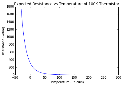

png

Now we can see that it does not have a linear relation. Actually it has a inverse relation or an $x^{n}$ where $n<0$ most probably. Since I am curious, I plotted the min and the max resistance to get a better feel for the error in the temperature reading. My ituition tells me that that is th range the thermister operates in.

plt.plot(data.temperature,data.r_norm, label='expected resistance')
plt.plot(data.temperature,data.r_min, label='min resistance')
plt.plot(data.temperature,data.r_max, label='max resistance')
plt.legend(bbox_to_anchor=(0., 1.02, 1., .102), loc=3,
           ncol=2, mode="expand", borderaxespad=0.)
plt.xlabel("Temperature (Celcius)")
plt.ylabel("Resistance (kohm)")
plt.title("Resistance vs Temperature of 100K Thermistor")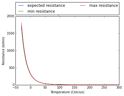

png

Now, the top graph, isn’t that useful. All it shows is that the range is very small, and is wider (there is more error) when temperatures are below 0 degrees. To see if we can do better, lets limit the range (with contingency) of the temperatures we will be dealing with on the project: 0-100 degrees.

plt.plot(data.temperature[30:130],data.r_norm[30:130], label='expected resistance')
plt.plot(data.temperature[30:130],data.r_min[30:130], label='min resistance')
plt.plot(data.temperature[30:130],data.r_max[30:130], label='max resistance')
plt.xlabel("Temperature (Celcius)")
plt.ylabel("Resistance (kohm)")
plt.legend(bbox_to_anchor=(0., 1.02, 1., .102), loc=3,
           ncol=2, mode="expand", borderaxespad=0.)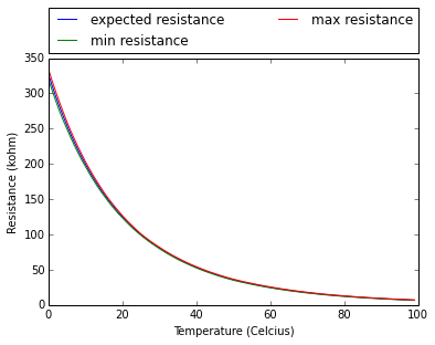

png

The plot is a bit clearer but not perfect, let’s try and be more fancy and reprensent the error with error bars like they do in stats 101.

data['lower_error'] = data.r_norm-data.r_min
data['upper_error'] = data.r_max-data.r_norm

asymmetric_error = [data.lower_error[30:130], data.upper_error[30:130]]
plt.errorbar(data.temperature[30:130], data.r_norm[30:130], yerr=asymmetric_error, ecolor='r')
plt.title("Resistance vs Temperature of 100K Thermistor")
plt.xlabel("Temperature (Celcius)")
plt.ylabel("Resistance (kohm)")
#plt.show()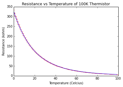

png

Great! A bit better, but it is still hard to read. Let’s try plotting the error on the same axis as the expected (normal) resistance.

plt.plot(data.temperature[30:130],data.r_min[30:130]-data.r_norm[30:130], label='lower error')
plt.plot(data.temperature[30:130],data.r_max[30:130]-data.r_norm[30:130], label='upper error')
plt.plot(data.temperature[30:130],data.r_norm[30:130], label='expected resistance')
plt.xlabel("Temperature (Celcius)")
plt.ylabel("Resistance (kohm)")
plt.legend(bbox_to_anchor=(0., 1.02, 1., .102), loc=3,
           ncol=2, mode="expand", borderaxespad=0.)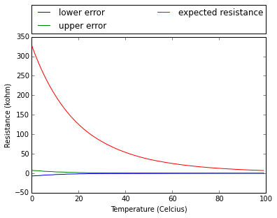

png

From this figure it is quite clear as tempertature decreases, there is more error in the thermistor reading. This figure also shows that reading taken over 20 C should have good accuracy. We can even take this futher by one more plot

plt.plot(data.temperature[50:130],data.r_min[50:130]-data.r_norm[50:130], label='lower error')
plt.plot(data.temperature[50:130],data.r_max[50:130]-data.r_norm[50:130], label='upper error')
plt.xlabel("Temperature (Celcius)")
plt.ylabel("Resistance (kohm)")
plt.legend(bbox_to_anchor=(0., 1.02, 1., .102), loc=3,
           ncol=2, mode="expand", borderaxespad=0.)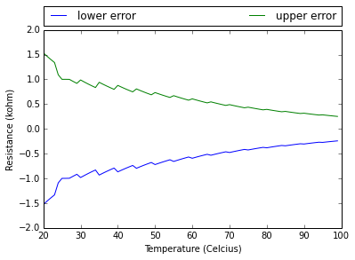

png

This figure shows the upper and lower bound of error (to be around $\pm 1.5k\Omega$)+ 125 kohm, since the expected reading would be around $125kOmega$ at 20 degrees C. Knowing the smallest resistance within our operating range will occur at 100 degrees (around $6720\Omega$), R_1 can be calculated to be around $1200\Omega$ using the voltage divider presented in the previous post. Now, the largest possible error can be calculated and used as a very conservative estime of the temperature reading resolution. Before we do that, let us fit a curve to the data. Using grade 11 math, we can estimate that the function which discribes the invest curve would look something like $resistance = a \times e^{-b \times temprature} + c$. We can then use SciPy’s curve_fit to determine the fit parameters and the covarience matrix.

def fitness_function(t, a, b, c):
    return a*np.exp(-b*t) + c
full_temp_fit_parms, full_temp_fit_covariances = curve_fit(fitness_function,
                                                           data.temperature, data.r_norm)
print ' full temperature fit coefficients:\n', full_temp_fit_parms
print ' Covariance matrix:\n', full_temp_fit_covariances

 full temperature fit coefficients:
[  3.22248984e+02   5.51886907e-02   4.56056442e+00]
 Covariance matrix:
[[  1.82147996e+00  -2.16345654e-04  -2.82466975e-01]
 [ -2.16345654e-04   2.97792772e-08   2.87522862e-05]
 [ -2.82466975e-01   2.87522862e-05   2.25733939e-01]]

The fit coefficients are now known! This means that the following equation approximates the behaviour of the thermister: $resistance = 322 \times e^{-0.055 \times temprature} + 4.56$

We can also determine the standard deviation of the fit from the diagonal of the covariance matrix, and plot it for each parameter.

# standard deviation of each paramter
sigma = [math.sqrt(full_temp_fit_covariances[0,0]), 
         math.sqrt(full_temp_fit_covariances[1,1]), 
         math.sqrt(full_temp_fit_covariances[2,2]) ]

x0 = np.linspace(300,340,1000)
x1 = np.linspace(0.05,0.06,1000)
x2 = np.linspace(2,7,1000)

fig = plt.figure(1)
plt.plot(x0,mlab.normpdf(x0,full_temp_fit_parms[0],sigma[0]))
plt.title("Uncertainty in fit parameter a")
plt.xlabel("Parameter a")
plt.ylabel("Standard Deviation")
fig = plt.figure(2)
plt.plot(x1,mlab.normpdf(x1,full_temp_fit_parms[1],sigma[1]), label='uncertainty in fit parameter b')
fig = plt.figure(3)
plt.plot(x2,mlab.normpdf(x2,full_temp_fit_parms[2],sigma[2]), label='uncertainty in fit parameter c')

#plt.show()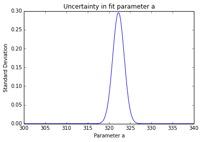

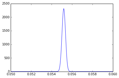
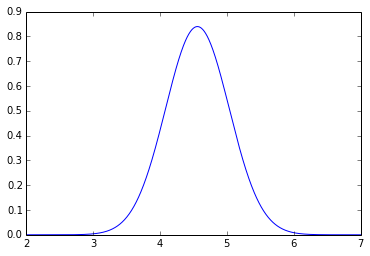
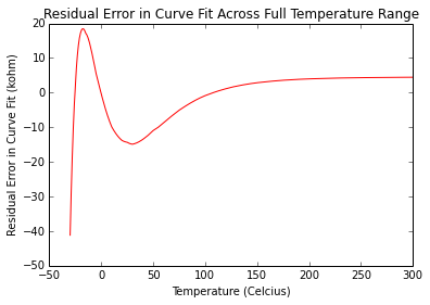
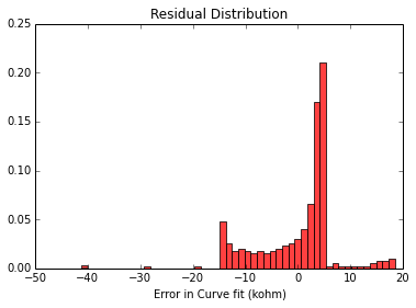
png

As we can see, the standard deviation is very small and thus results in a good fit accross the full range of temperature as shown in the three figures below:

full_temp_fit = fitness_function(data.temperature,
                                 full_temp_fit_parms[0],
                                 full_temp_fit_parms[1],
                                 full_temp_fit_parms[2])
residual_error= full_temp_fit -data.r_norm

plt.figure(1)
plt.plot(data.temperature,full_temp_fit,label='curve fit')
plt.plot(data.temperature,data.r_norm, label='expected')
plt.plot(data.temperature,residual_error, label='residual error')
plt.legend(bbox_to_anchor=(0., 1.02, 1., .102), loc=3,
           ncol=2, mode="expand", borderaxespad=0.)
plt.xlabel("Temperature (Celcius)")
plt.ylabel("Resistance (kohm)")
plt.title("Resistance vs Temperature of 100K Thermistor")

plt.figure(2)
plt.plot(data.temperature,residual_error, 'r', label='residual error')
plt.xlabel("Temperature (Celcius)")
plt.ylabel("Residual Error in Curve Fit (kohm)")
plt.title("Residual Error in Curve Fit Across Full Temperature Range")

plt.figure(3)
n, bins, patches = plt.hist(residual_error, 50, normed=1, facecolor='red', alpha=0.75)
plt.xlabel("Error in Curve fit (kohm)")
plt.title("Residual Distribution")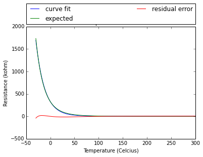

png

While the model accross the full temperature is useful, we can improve our model by curve fitting only in the temperature range we are interested in. This prevents the algorithm for compesating for select set of data which is irrevant.

#temperature ranger 0 to 100 degrees
selected_temp = data.temperature[30:130]
selected_r_norm = data.r_norm[30:130]
selected_temp_fit_parms, selected_temp_fit_covariances = curve_fit(fitness_function,
                                                    selected_temp, selected_r_norm)
print ' fit coefficients:\n', selected_temp_fit_parms
print ' Covariance matrix:\n', selected_temp_fit_covariances

selected_temp_fit = fitness_function(selected_temp,
                                 selected_temp_fit_parms[0],
                                 selected_temp_fit_parms[1],
                                 selected_temp_fit_parms[2])
residual_error_selected = selected_temp_fit-selected_r_norm

plt.figure(1)
plt.plot(selected_temp, selected_temp_fit,label='curve fit')
plt.plot(selected_temp, selected_r_norm, label='expected')
plt.plot(selected_temp,residual_error_selected, 'r' , label='residual error')
plt.legend(bbox_to_anchor=(0., 1.02, 1., .102), loc=3,
           ncol=2, mode="expand", borderaxespad=0.)
plt.xlabel("Temperature (Celcius)")
plt.ylabel("Resistance (kohm)")

plt.figure(2)
plt.plot(selected_temp,residual_error_selected, 'r' , label='residual error')
plt.xlabel("Temperature (Celcius)")
plt.ylabel("Residual Error in Curve Fit (kohm)")
plt.title("Residual Error in Curve Fit Across Full Temperature Range")

plt.figure(3)
# convert numpy series to array
residual_error_list  = residual_error_selected.tolist()
residual_error_array = np.asarray(residual_error_list)

n, bins, patches = plt.hist(residual_error_array, 50, normed=1, facecolor='red', alpha=0.75)
plt.xlabel("Error in Curve fit (kohm)")
plt.title("Residual Distribution")

 fit coefficients:
[  3.16643400e+02   4.84933743e-02   6.53548105e+00]
 Covariance matrix:
[[  3.29405526e-01   4.07305280e-05  -1.67742297e-02]
 [  4.07305280e-05   3.89687128e-08   4.14707796e-05]
 [ -1.67742297e-02   4.14707796e-05   7.51633680e-02]]

png

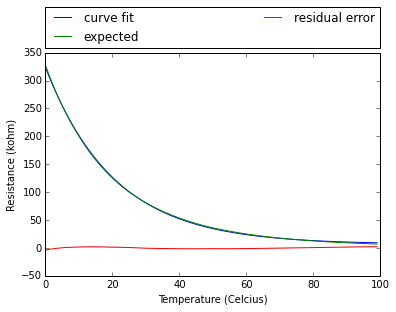
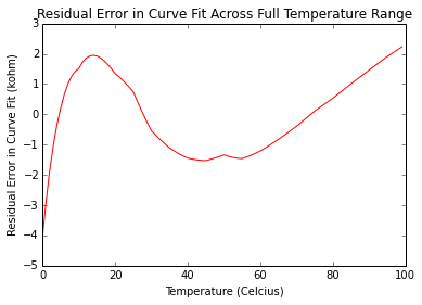
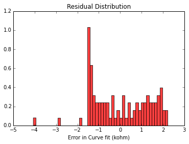
We can see the difference by comparing both of the curve fit models on the interested temperature range:

While the testing spec we developed states we should have the capability of measuring from 0-100 degress C, the average range of operation is actually between 20-80 degrees C, so we can change the range to match the standard operating range

#temperature ranger 0 to 100 degrees
selected_temp = data.temperature[50:110]
selected_r_norm = data.r_norm[50:110]
selected_temp_fit_parms, selected_temp_fit_covariances = curve_fit(fitness_function,
                                                    selected_temp, selected_r_norm)
print ' fit coefficients:\n', selected_temp_fit_parms
print ' Covariance matrix:\n', selected_temp_fit_covariances

selected_temp_fit = fitness_function(selected_temp,
                                 selected_temp_fit_parms[0],
                                 selected_temp_fit_parms[1],
                                 selected_temp_fit_parms[2])
residual_error_selected = selected_temp_fit-selected_r_norm

plt.figure(1)
plt.plot(selected_temp, selected_temp_fit,label='curve fit')
plt.plot(selected_temp, selected_r_norm, label='expected')
plt.plot(selected_temp,residual_error_selected, 'r' , label='residual error')
plt.legend(bbox_to_anchor=(0., 1.02, 1., .102), loc=3,
           ncol=2, mode="expand", borderaxespad=0.)
plt.xlabel("Temperature (Celcius)")
plt.ylabel("Resistance (kohm)")

plt.figure(2)
plt.plot(selected_temp,residual_error_selected, 'r' , label='residual error')
plt.xlabel("Temperature (Celcius)")
plt.ylabel("Residual Error in Curve Fit (kohm)")
plt.title("Residual Error in Curve Fit Across Full Temperature Range")

plt.figure(3)
# convert numpy series to array
residual_error_list  = residual_error_selected.tolist()
residual_error_array = np.asarray(residual_error_list)

error_mean = np.mean(residual_error_array)
error_sigma = np.std(residual_error_array)
print "Residual mean (Kohm):"
print error_mean
print "Residual std dev (Kohm):"
print error_sigma


n, bins, patches = plt.hist(residual_error_array, 50, normed=1, facecolor='red', alpha=0.75)
plt.xlabel("Error in Curve fit (kohm)")
plt.title("Residual Distribution")
y = P.normpdf( bins, error_mean, error_sigma)
l = P.plot(bins, y, 'k--', linewidth=1.5)

 fit coefficients:
[  2.94311453e+02   4.51009053e-02   5.05438839e+00]
 Covariance matrix:
[[  6.57786227e-01   1.12143572e-04   8.24269669e-02]
 [  1.12143572e-04   2.18837795e-08   1.84056321e-05]
 [  8.24269669e-02   1.84056321e-05   1.81122519e-02]]
Residual mean (Kohm):
9.99334067349e-10
Residual std dev (Kohm):
0.2302444024

png

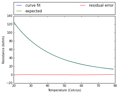
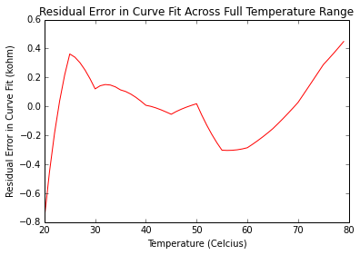
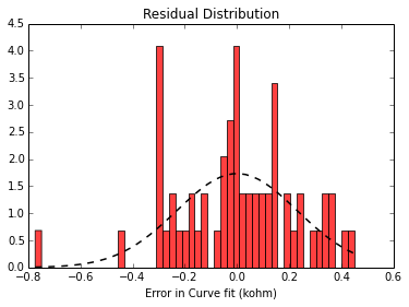
The results of the curve fit within the standard operating temperature is much better. Now only is residual error mean essentually zero (9.99e-10 k ohm) with a relatively small standard deviation (0.230 kohm), but the residual error have the general appearance of being normally distributed (unlike the previous curve fits). What this means is that, the model will predict the resistance very well (have a very low error) for the stardard operating temperatures, but will perform poorer outside. Luckly for us, our battries will not be operating below 20 degrees C or above 80 degrees C.

Curve fit model:

The model we created can now be sumarized to the following equation:

$R_2 = a e^{-b \times temperature} + c$ where R_2 is meaured in $k\Omega$, temperature measued in degree celcius, and the constants a, b, and c were found (through curve fitting) to be:

$a = 2.94311453 \times 10^2$
$b = 4.51009053 \times 10 ^{-02}$
$c = 5.054388390$

In addition, the error in the curve fitting is averaged at 9.99334067349e-10 kohm and the standard deviation of 0.2302444024 kohm. This error, while small can later be used in filtering algorithms when we are monitoring the temperature. I will touch on this in a later post, but this data about statistical noise while reading can aid in estimating temperature through more advance software (such as using Kalman Filtering).

Writing software to convert voltage into temperature readings

If we think of the system as a whole, the input to the system is Vo which is measured on an analog input pin of the BBB. Based on this voltage reading, we have to write software which estimates the temperature.

To begin, we know that the thermister (R_2) changes resistance values depending on temperature. We can then use the voltage devider to map this relation:

\[V_o = \frac{R_2 V_{in}}{R_1 + R_2}\]

Vin in this case will be 3.3 V which is provided from the BBB. As noted in the last post, the spec on the BBB states that that analog input pin can only take in voltage in the range of 0 to 1.8 V. This means we can set the max Vout = 1.8. Finally based on the resistance to temperature data, we know that resistance increases as the temperature decreases. This means that R_2 (the resistance of the thermistor), will be the greatest when T = 0 degrees (R_2 will be around 327 kohms. We can then use this in our voltage divider equation and solve for R_1. The solution is R_1 = 272700 ohms. Because resistors come in standard sizes, 274K ohm is the stardard 1% error resistor to use. Technically, in this case we should go to the next highest resistor value (to limit the voltage to 1.8V), this doesn’t necessarily have to be true since we will not be cooling the batteries lower than room temperature. While I recommend using the 274k ohm resistor (with 1% error), one can use a 270k ohm (with 5% error) without much concequece if they ensure that the temperature does not fall below 5 degrees. Even if it does, the Beaglebone has some circuity to help prevent damamge for a slightly larder analog input voltage.

We can use algebra to solve for R_2 in terms of the other variables as the following:

$R_2 = \frac{R_1 V_o}{V_{in} - V_o}$ where $V_{in} \neq V_o$

In this equation, R_2 can be solved from R_1 (set by us, V_o (measured), V_in (set to by us).

Next we can use the previous curve fit equation, and use algebra solve for temperature:

$temperature = - \frac{ln (\frac {R_2-c}{a}}{b}$ where $R_2 > c$$$

We can then substitute our relation of R_2 to the measured Vo to get the following equation:

$temperature = -ln (\frac {\frac{R_1 V_o}{V_{in} - V_o}-c}{ab}$ where $R_2 > c$ and $V_{in} \neq V_o$$$

Before we can use this, we have to ensure the conditions hold. V_o will on equal V_in if R_2 is equal to zero, and we also ensure C (about 5.5 kohm) > R_2. If we use the data found in the csv, we see that the smallest resistance in our operaterting temperature (100 C) is 6.7100 kohm, so we are safe for both conditions.

Results!

We can now write a simple which takes the a volatage as a parameter, and returns the temperature.

def voltage_to_temperature(voltage_reading):
    r_1 = 274 #kohm
    v_in = 3.3 #Volts
    a = 2.94311453*pow(10,2)
    b = 4.51009053*pow(10,-2)
    c = 5.054388390
    
    r_2 = r_1 * voltage_reading / (v_in - voltage_reading) # kohm
    
    t = -1 * (np.log((r_2-c)/a))/b
    return t
print voltage_to_temperature(1.8)

-2.11347171107

We can now use this function and plot for the full range of input voltages:

v_sweep = np.linspace(0, 1.8, num=1000)
temperature_profile = voltage_to_temperature(v_sweep)

plt.plot(v_sweep, temperature_profile)
plt.ylabel("Temperature (Celcius)")
plt.xlabel("Measured Voltage (V)")
plt.title("Temperature vs Measured Voltage")

Using this chart we can now test the system and measure temperature! The next post will be about combining all the prieces and doing the testing!

Modeling a Thermister: Merging Hardware Engineering and Data Science Curve fitting, residuals and fun math!